Differentiable Unconstrained Minimization
minsubject tof(x)x∈Rn
其中f可微
Convergence Rate
计算方法:
假设给定objective function能够转换成一个序列rk, 计算极限
q=k→∞limrkrk+1
convergence rate就是q.
Convergence Type
- q=0: superlinearly
- 0<q<1: linearly
- q=1: sublinearly
- q>1: non-convergence
假设λ1(Q)是Q的最大的eigenvalue, λn(Q)是最小eigenvalue, 那么可以认为:
r=λn(Q)λ1(Q)=minxλn(∇2f(x))maxxλ1(∇2f(x))
ηt≡η=λ1(Q)+λn(Q)2, 那么
∥xt−x∗∥2≤(λ1(Q)+λn(Q)λ1(Q)−λn(Q))t∥x0−x∗∥2=ε
Convergence Analysis:
1.2.3.∥xt−x∗∥2≤ε∥f(xt)−f(x∗)∥2≤ε∥∇f(x)∥2≤ε
Convergence Rate:
- sublinear: T>εk1,o(εk1)
- linear: T>logε1,o(logε1)
- quadratic(super linear): T>log(logε1),o(log(logε1))
Iteration Function:
4. sublinear: ∥xt−x∗∥2≤tk11∥x0−x∗∥2
5. linear: ∥xt−x∗∥2≤∥xq−1−x∗∥2⇒∥xt−x∗∥2≤qt∥x0−x∗∥2
6. quadratic: ∥xt−x∗∥2≦∥xq−1−x∗∥22
Iterative descend algorithm
从x0开始, 构造序列{xt}满足f(xt+1)<f(xt),t=0,1,⋯
下降方向(descend direction) d 满足:
f′(x;d):=τ↓0limτf(x+τd)−f(x)=∇f(x)⊤d≤0
每一次迭代中, 有xt+1=xt−ηdt, 其中dt是在xt的时候的descend direction, η是步长.
在机器学习中, f通常是loss函数, x通常是loss函数中的参数, η是学习率
Steepest Descend 最陡下降法
- 最快优化objective function的方向:
mathop{\arg\min}_{\mathbf d:|\mathbf d|2\leq1}f’(\mathbf x;\mathbf d)=\mathop{\arg\min}{\mathbf d:|\mathbf d|_2\leq1}\nabla f(\mathbf x)^\top\mathbf d=-|\nabla f(\mathbf x)|_2$$
−∥∇f(x)∥⋅∥d∥2≤⟨∇f(x),d⟩≤∥∇f(x)∥⋅∥d∥2
Quadratic Minimization
minsubject tof(x):=21(x−x∗)⊤Q(x−x∗)Q≻0
该方程的梯度为∇f(x)=Q(x−x∗)
参数更新:
xt+1=(I−ηtQ)xt+ηtQx∗
step size(η) rule:
⇒⇒⇒xt+1−x∗=(I−ηtQ)(xt−x∗)∥xt+1−x∗∥≤∥I−ηtQ∥⋅∥xt−x∗∥∥I−ηQ∥=λ1(Q)+λn(Q)λ1(Q)−λn(Q)η≡ηt=λ1(Q)+λn(Q)2
Exact Line Search
ηt=argminη≥0f(xt−η∇f(xt))
假设有gt=∇f(xt)=Q(xt−x∗), 那么ηt=gt⊤Qgtgt⊤gt
Kantorovich’s inequality:
(y⊤Qy)(y⊤Q−1y)∥y∥24≥(λ1(Q)+λn(Q))24λ1(Q)λn(Q)
Smooth problem
μ-strong和L-smooth定义:
0⪯μI⪯∇2f(x)⪯LI
或者:
λn(Q)I⪯Q⪯λ1(Q)I
对于μ-strong和L-smooth的问题, 有:
- step size: η=μ+L2 (v.s. λ1+λn2)
- contraction rate: κ+1κ−1,κ=μL (v.s. λn+λ1λ1−λn)
iteration complexity: o(logκ+1κ−1logε1)
f(xt)−f(x∗)≤2L(κ+1κ−1)2t∥x0−x∗∥2
Backtracking Line Search
Armijo Condition:
f(xt−η∇f(xt))<f(xt)−αη∥∇f(xt)∥22,0<α<1
algorithm:
- initialize η=1, 0<α<21, 0<β<1
- while f(xt−η∇f(xt))<f(xt)−αη∥∇f(xt)∥22, do:
上界: f(xt)−η∥∇f(xt)∥22+2Lη2∥∇f(xt)∥22
f(xt)−f(x∗)≤(1−min{2μα,L2βαμ})t(f(x0)−f(x∗))
收敛性:
∥xt−x∗∥≤κ+1κ−1∥xt−1−x0∥
Regularity Condition
μ-strong + L-smooth
η≡ηt=L1
∥xt−x∗∥≤(1−Lμ)t∥x0−x∗∥
Polyak-Lojasiewicz Condition
∥∇f(x)∥22≥2μ(f(x)−f(x∗))
f(xt)−f(x∗)≤(1−Lμ)t(f(x0)−f(x∗))
Over-parameterized linear regression
over-parameterize: model dimension > sample size
定义
f(x)=21i=1∑m(ai⊤x−yi)2=21(AX−Y)2
有
∇f(x)=0⇔X=(A⊤A)−1A⊤Y
∇2f(x)=i=1∑maiai⊤
认为如果A=[a1,⋯,am]⊤∈Rm×n, 其rank为m, 且满足step size ηt≡η=λmax(AA⊤)1, 有:
f(xt)−f(x∗)≤(1−λmax(AA⊤)λmin(AA⊤))t(f(x0)−f(x∗)),∀t
Convex and Smooth Problem
L-smooth
majorization-minimization
如果是L-smooth的, 且有: η=L1
f(xt+1)≤f(xt)−2L1∥∇f(xt)∥22
∥xt−x∗∥≤∥xt−1−x∗∥−L21∥∇f(xt−1)∥22
f(xt)−f(x∗)≤t2L∥x0−x∗∥
Non-convex Problem
- for general: $min0≤k<t∥∇f(xk)∥2≤t2L(f(x0)−f(x∗))$
- for convex: $min2t≤k<t∥∇f(xk)∥2=t4L∥x0−x∗∥2$
Gradient methods for Constrained Problems
Frank-Wolfe algorithm
- yt:=argminx∈C⟨∇f(xt),xt⟩
- xt+1=(1−ηt)xt+ηtyt
over a convex set: f(xt)+⟨∇f(xt),x−xt⟩. 步长类似Exact Line Search: ηt=t+22
对于non-convex:
minimizesubject to−x⊤Qx∥x∥2≤1
有:
yt⇒xt+1=argminx:∥x∥2≤1⟨∇f(xt),x⟩=−∥∇f(xt)∥2∇f(xt)=∥Qxt∥2Qxt=(1−ηt)xt+ηt∥Qxt∥2Qxt
Convergence
假设f是convex的, 且是L-smooth的, 假设有ηt=t+22, 那么有:
f(xt)−f(x∗)≤t+22LdC2
其中dC=supx,y∈C∥x−y∥2
对于compact约束集合, 效率可以达到 ε-accuracy, 在O(ε1)个迭代中
假设有集合C是μ-convex的, 假设∀λ∈[0,1], ∀x,z∈C, 定义B(a,r):={y∣∥y−a∥2≤r}, 那么有:
B(λx+(1−λ)z,2μλ(1−λ)∥x−z∥22)∈C
假设f是convex and L-smooth的, 假设C是μ-strongly convex的, 那么0≤c≤∥∇f(x)∥2,∀x∈C
Projected Gradient Method
将一个在集合外的点映射到集合中
Euclidean projection(quadratic minimization):
PC(x):=argminz∈C∥x−z∥22
循环:
xt+1=PC(xt−ηt∇f(xt))
假设有集合C是close且convex的, 那么有:
(x−PC(x))⊤(z−PC(x))≤0,∀z∈C
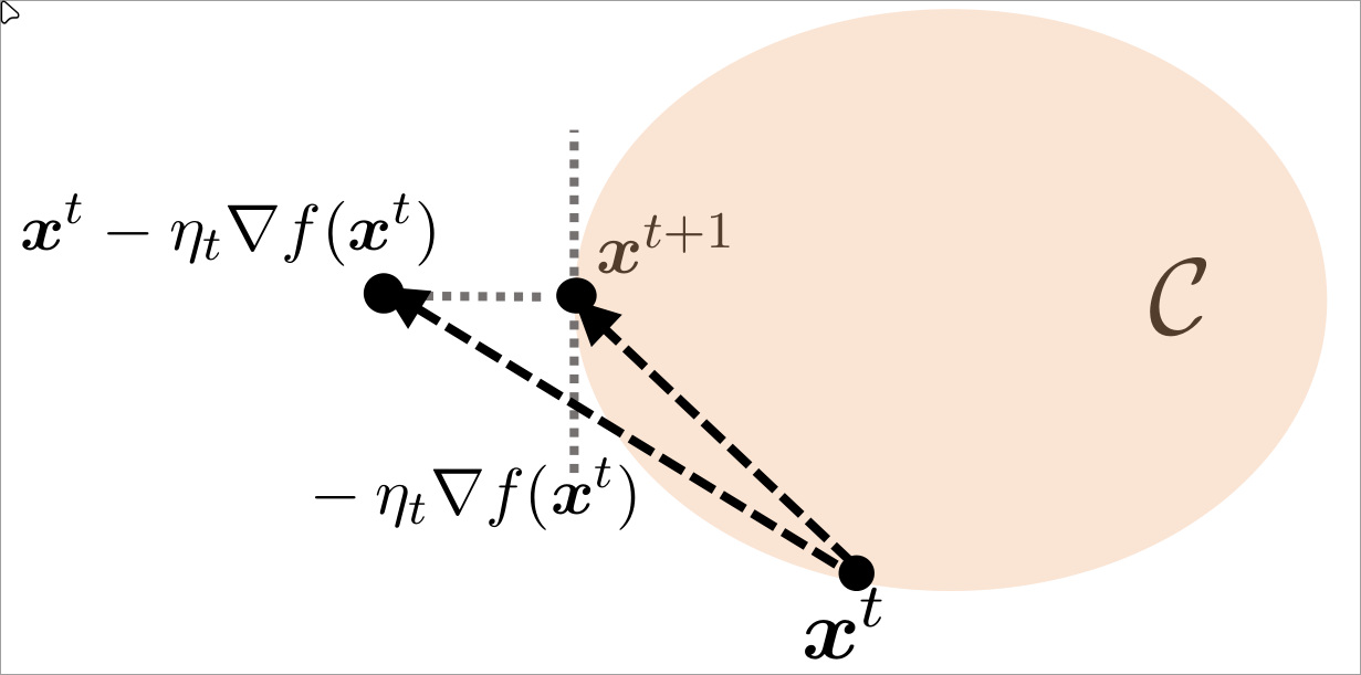
从上图可知, 有−∇f(xt)⊤(xt+1−xt)≥0, 即xt+1−xt和最速下降的方向是正相关的
Strongly Convex
假设x∗∈int(C), 假设f是μ-strongly convex且L-smooth的. 令ηt=μ+L2,κ=μL, 有
∥xt−x∗∥2≤(κ+1κ−1)t∥x0−x∗∥2
一些其他情况参见Smooth problem